#1 Classification: VGG19 on CIFAR100
This page introduces how Nota could compress and optimize the VGG19 model with NetsPresso Model Compressor and Nota’s unique search algorithm.
Preparations
Let's briefly explain the input model and training details used in the example.
1) Model & Training Code
- Data: CIFAR100
- Model: VGG19 (TensorFlow)
Model and training code are in the [NetsPresso Model Compressor ModelZoo] (https://github.com/Nota-NetsPresso/NetsPresso-CompressionToolkit-ModelZoo/tree/main/models/tensorflow).
Training code is required to fine-tune the model after compression.
2) Train Config
The following table describes the configurations for training:
| Parameter | Value |
|---|---|
| Normalization | Mean: [0.4914, 0.4822, 0.4465] SD: [0.2023, 0.1994, 0.2010] |
| Data Augmentation | RandomCrop(32, padding=4), RandomHorizontalFlip |
| Learning Rate | 0.01 |
| Optimizer | SGD (momentum: 0.9) |
| Batch size | 128 |
| Epochs | 100 |
| LR Scheduler | ReduceLROnPlateau |
Simple Compression

Stage 1: Filter Decomposition
First, we adopted a Filter Decomposition (FD). The aim of FD is to approximate the original filter's representation with fewer filters (ranks).
Since each layer has different amounts of information, finding an optimum rank for each layer is crucial to minimize the accuracy drop.
Please refer to the attached document if you would like to learn more about FD.
Netspresso Model Compressor offers you two options to implement FD:
- Use our recommended values (automatically calculated)
- Use your own values (customized)
Recommendation function, based on VBMF, presents the optimal rank for each layer in a minute.
1) Tucker Decomposition
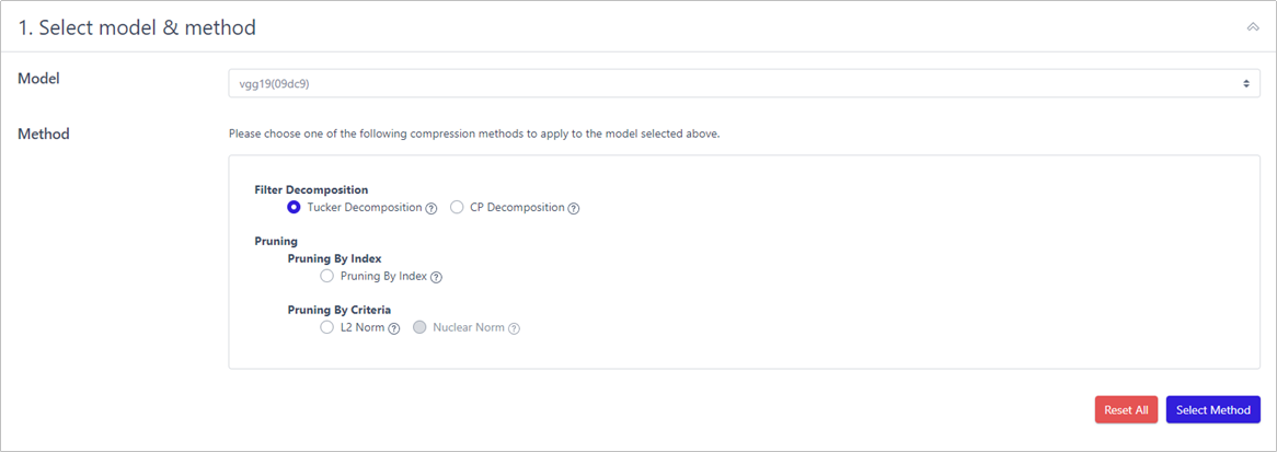
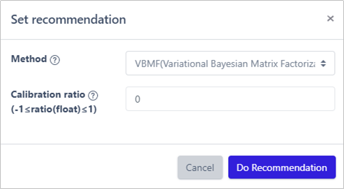
Calibration ratio allows a user to easily increase or decrease filter's rank to search for a better performing model. The new rank is calculated by adding (removed rank x calibration ratio) to the remained rank. The ratio is set to 0 as default.
More detailed information can be found at Calibration Ratio Description.
This is what you will see when you click the Recommendation button.

Why there is no recommendation for the first layer?
It is because "In Channel" of the first layer is 3, so there is not much information.
Recommendation function automatically excludes such layers to avoid significant drop in accuracy.
2) Fine-tuning
After the compression, a model culminates in a significant performance deterioration. Thus, fine-tuning is an essential process to recover the original performance.
To fine-tune the model, run the train code we provided NetsPresso Model Compressor ModelZoo.
Make sure that the training config for fine-tuning is exactly same with the one for an original model.
Stage 2: Pruning
Now, we prune a model to further lighten the model. The goal is to reduce the computational resources and accelerate the model by removing less important and redundant filters.
Please refer to the attached document if you would like to learn more about pruning.
Since there is a huge variation in layers' significance, the performance of a model may fluctuate dramatically depending on which filter is removed.
Just like FD, NPTK offers two options to implement pruning:
- Use our recommended values (automatically calculated)
- Use your own values (customized)
Recommendation function, based on SLAMP, presents the pruning ratio for each layer in a few seconds.
1) L2 Norm
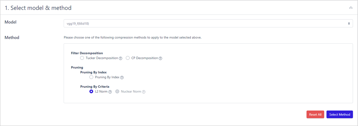

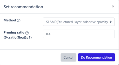
Pruning ratio is how much filters to be pruned. As shown above, pruning_ratio=0.4 means to remove 40% of the network.
2) Fine-tuning
As we did after FD, we fine-tuned the model after pruning it.
It can be done using the training code provided. Again, make sure that the training config for fine-tuning is exactly same with the one for an original model.
Result of Compression
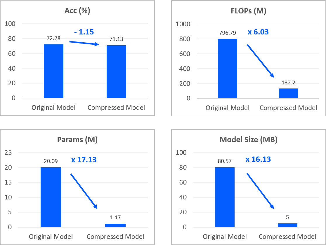
| Name | Acc (%) | FLOPs (M) | Params (M) | Model Size (MB) |
|---|---|---|---|---|
| Original | 72.28 | 796.79 | 20.09 | 80.57 |
| FD | 71.64 (-0.64) | 156.30 (5.1x) | 1.69 (11.9x) | 7.08 (11.38x) |
| FD + Pruning | 71.13 (-1.15) | 132.20 (6.03x) | 1.17 (17.13x) | 5.00 (16.13x) |
Search-Based Compression
To achieve the best, we utilized our own unique in-house search algorithm to find better compression parameters (rank & pruning ratio).
Unfortunately, the algorithm is only for internal usage and not provided in this trial version. If you are interested in our solution, please reach out to us.
The figure below illustrates our procedure.

The compression parameters obtained from our search algorithm are listed below. Using the parameters, you are able to create a model with the same performance.
Why is there a difference in performance between mine and Nota's?
Due to stochastic causes, fine-tuning may lead to a minor variance in accuracy.
Stage 1: Filter Decomposition
1) FD Compression Parameter
# layer name : [In Rank, Out Rank]
'features.3': [33, 39]
'features.7': [40, 54]
'features.10': [54, 51]
'features.14': [67, 89]
'features.17': [107, 103]
'features.20': [106, 110]
'features.23': [104, 97]
'features.27': [130, 182]
'features.30': [220, 183]
'features.33': [87, 78]
'features.36': [75, 86]
'features.40': [64, 69]
'features.43': [64, 72]
'features.46': [72, 97]
'features.49': [143, 191]
Stage 2. Pruning
1) Pruning Compression Parameter
# layer name : Pruning Ratio
'features.0': 0.5
'features.3_tucker_0': 0.5
'features.3_tucker_1': 0.3
'features.3_tucker_2': 0.0
'features.7_tucker_0': 0.4
'features.7_tucker_1': 0.3
'features.7_tucker_2': 0.0
'features.10_tucker_0': 0.2
'features.10_tucker_1': 0.1
'features.10_tucker_2': 0.0
'features.14_tucker_0': 0.3
'features.14_tucker_1': 0.1
'features.14_tucker_2': 0.0
'features.17_tucker_0': 0.2
'features.17_tucker_1': 0.1
'features.17_tucker_2': 0.0
'features.20_tucker_0': 0.1
'features.20_tucker_1': 0.2
'features.20_tucker_2': 0.0
'features.23_tucker_0': 0.4
'features.23_tucker_1': 0.2
'features.23_tucker_2': 0.0
'features.27_tucker_0': 0.5
'features.27_tucker_1': 0.5
'features.27_tucker_2': 0.2
'features.30_tucker_0': 0.8
'features.30_tucker_1': 0.9
'features.30_tucker_2': 0.7
'features.33_tucker_0': 0.9
'features.33_tucker_1': 0.9
'features.33_tucker_2': 0.6
'features.36_tucker_0': 0.9
'features.36_tucker_1': 0.9
'features.36_tucker_2': 0.4
'features.40_tucker_0': 0.9
'features.40_tucker_1': 0.9
'features.40_tucker_2': 0.8
'features.43_tucker_0': 0.9
'features.43_tucker_1': 0.9
'features.43_tucker_2': 0.7
'features.46_tucker_0': 0.9
'features.46_tucker_1': 0.8
'features.46_tucker_2': 0.5
'features.49_tucker_0': 0.9
'features.49_tucker_1': 0.8
'features.49_tucker_2': 0.3
Result of Compression
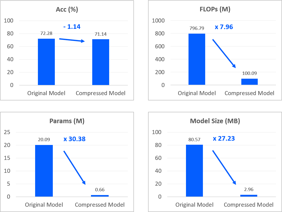
| Name | Acc (%) | FLOPs (M) | Params (M) | Model Size (MB) |
|---|---|---|---|---|
| Original | 72.28 | 796.79 | 20.09 | 80.57 |
| FD | 71.64 (-0.64) | 206.95 (3.85x) | 2.67 (7.52x) | 11.02 (7.31x) |
| FD + Pruning | 71.14 (-1.14) | 100.09 (7.96x) | 0.66 (30.38x) | 2.96 (27.23x) |
NPTK-Simple vs NPTK-Search
The results from Nota-Simple and Nota-Search
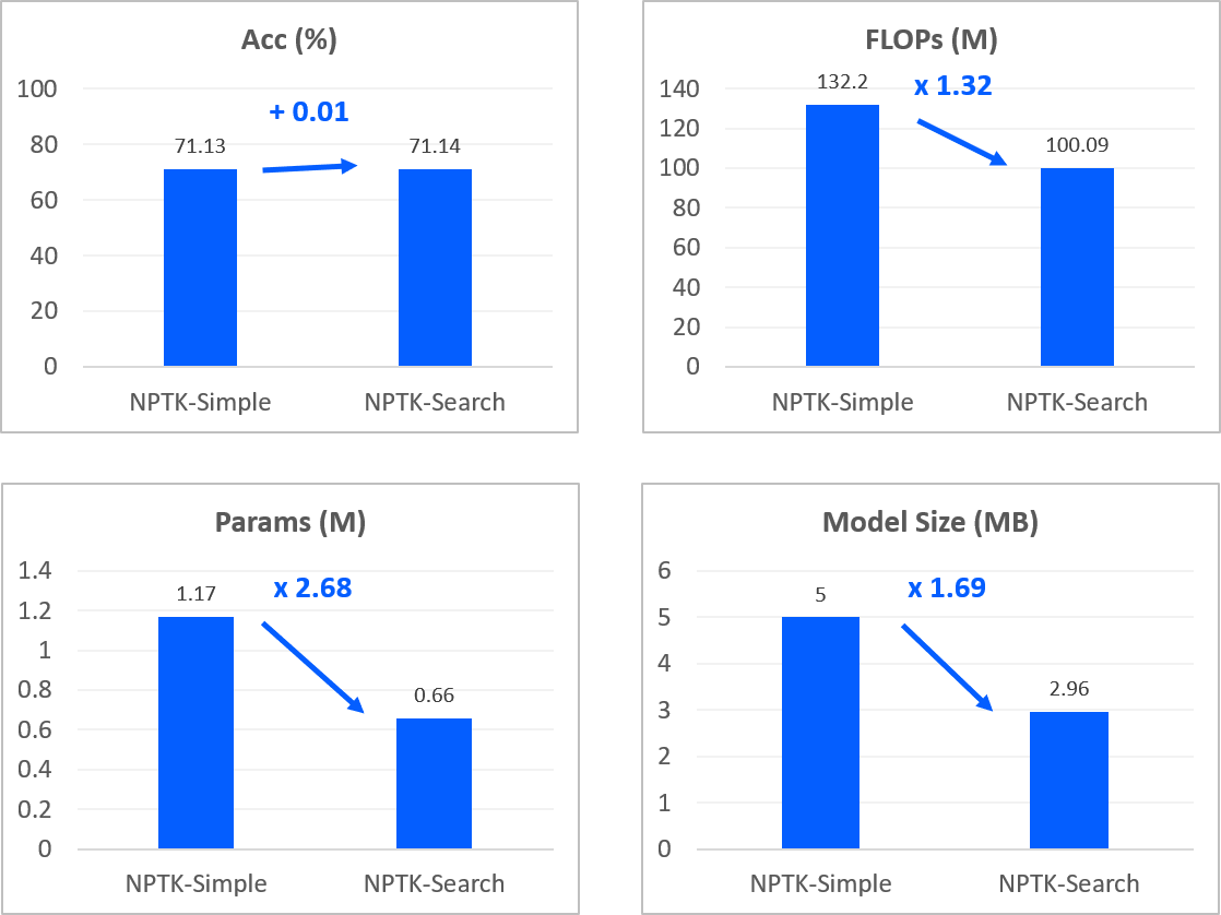
Summary
We have walked you through how we could compress a CNN model with NetsPresso Model Compressor. You could see how Model Compressor reduced FLOPs, parameters, and a model size while maintaining the accuracy of an original model.
There are more blogs coming - object detection, super resolution. To stay up to date, sign up or subscribe at netspresso.ai.
Updated almost 2 years ago
